Chapter 3 Maps and spatial data for communities connected to public sewer
3.1 Overview
In this section, we will review existing maps for community sewer and how to go about making them. While there is a plethora of digital spatial data on many topics, there is not yet a comprehensive national database for sewers in the United States (US). Prior to the NYS DOH sewershed mapping project, there was also not a comprehensive map of NY’s sewer systems. There are, however, some public databases for locations of publicly owned treatment works including permitted wastewater treatment plants. The US Environmental Protection Agency (EPA) maintains records on permitted WWTPs and so do most state environmental offices. Using these public records, we know where the municipal WWTPs are and this provides a starting point for mapping a state’s sewer systems. The next step involves collecting data from other sources like:
- State tax parcel records
- Municipal records for local sewer taxes
- WWTP infrastructure maps or engineering design
- County or local planning documents
- Location of manholes or sewer mains
- Lists of addresses for properties that report paying a sewer tax
Many of these records will be housed in local GIS, tax, planning, or municipal offices. Some will be public, and others might require permission to access or data use agreements. The final product of mapping a state’s sewer systems does not result in any identifiable data being produced, and if you explain to local officials the goals of the project and what the final product will look like, data sharing should not be an issue. Work with your local partners to ensure that their questions are answered, and any concerns are addressed.
3.2 Goals for this section
In this section, you will:
- Review an example sewershed parcel mapping exercise for one county in New York State
- Explore loading and manipulating maps in ArcGIS and R
- Gather data on your state’s WWTP locations
- Contact local offices, WWTP operators, and others to gather data on sewer locations
- Gather parcel property data for your jurisdiction
3.3 Resources
- National parcel data viewer / data access portal. This is a data portal that lets you explore each state in the US and whether they have tax parcel data. Some links bring you to county or state websites and from there you can view and download the data.
ArcGIS tutorials
Q GIS tutorials
3.4 Training exercise
This training will show how to use publicly available tax parcel data to draw municipal sewershed boundaries. You will need to download R to run this script on your machine.
For this example, we are going to map sewersheds in Onondaga County, NY. Sewersheds are the area of land that a wastewater treatment plant (WWTP) serves and include public and private properties. Many states, including NY, keep track of residential and commercial sewer access in their state tax records. We will use data downloaded from the NYS Tax Parcel system for Onondaga county.
You can access the file for Onondaga County at the following location: NYS Tax Parcel Data. These data are very large, so for the purposes of this tutorial, I have already downloaded the data and filtered for Onondaga County.
You will also need a list of the municipal wastewater treatment plants for Onondaga County. NYS keeps a record of all permitted WWTPs in the state. You can download the file here.
We will be able to use these data to:
Map WWTPs in Onondaga County, NY
Select parcels that are on public sewer
Link groups of parcels to the town or village they are within
Estimate sewershed locations for nearby WWTPs
A note before proceeding: Parcel data are very large and your R session might slow down during some processing steps.
3.4.0.1 Data you will need for this tutorial
You will need to download the following data files for this tutorial (they are stored with this tutorial).
Onondaga County tax parcels
NYS WWTP list
NY county boundaries
NY town boundaries
NY village boundaries
3.4.1 Step 1 - Install and load the necessary R packages
Install packages to your computer.
install.packages("gridExtra")
install.packages("nngeo")
install.packages("sf")
install.packages("dplyr")
install.packages("ggplot2")
install.packages("tigris")
Load packages into your current R session.
library(gridExtra)
library(nngeo)
library(sf)
library(dplyr)
library(ggplot2)
library(tigris)
3.4.2 Step 2 - Load the data into your R session
# Onondaga county tax parcels
onondaga_parcels <-
  st_read("E:/Data/ny_parcels/onondaga_2020_Tax_Parcels_SHP_2106/onondaga_2020_Tax_Parcels_SHP_2106.shp")

# NY WWTPS
ny_wwtps <- read.csv("data/Wastewater_Treatment_Plants_20250121.csv")

# NY county boundaries - for assistance with mapping
ny_counties <-
  st_read("E:/Dropbox/CEMI/Wastewater/Data/NYS_Civil_Boundaries.shp/Counties_Shoreline.shp")

# Filter for Onondaga county
onondaga_border <- ny_counties %>%
  filter(NAME == "Onondaga")

# nys town, city, village boundaries
towns <-
  st_read("E:/Dropbox/CEMI/Wastewater/Data/NYS_Civil_Boundaries.shp/Cities_Towns.shp")

# Onondaga towns
onondaga_towns <- towns %>%
  filter(COUNTY == "Onondaga")

# villages
villages <-
  st_read("E:/Dropbox/CEMI/Wastewater/Data/NYS_Civil_Boundaries.shp/Villages.shp")

# Onondaga villages
onondaga_villages <- villages %>%
  filter(COUNTY == "Onondaga")
3.4.3 Step 3 - Filter the WWTP data for municipal sites only
# municipal sites only
wwtp_mun <- ny_wwtps %>%
  filter(Plant.Type == "Municipal")

# make the data spatial for mapping purposes using the coordinates in the file
wwtp_mun_sf <-
  st_as_sf(wwtp_mun,
           coords =  c("Longitude", "Latitude"),
           crs = "+proj=longlat +datum=WGS84 +no_defs +ellps=WGS84")

# transform to the same CRS as the Onondaga parcels
wwtp_mun_sf <- st_transform(wwtp_mun_sf, st_crs(onondaga_border))

# filter for Onondaga plants only using st_intersection
wwtp_onondaga_sf <- st_intersection(wwtp_mun_sf, onondaga_border)

# Map out the plants
ggplot()+
  geom_sf(data = onondaga_border, fill = NA)+
  geom_sf(data = onondaga_towns, fill = "dodgerblue", color = "white")+
  geom_sf(data = onondaga_villages, fill = "orange", color = "white")+
  geom_sf(data = wwtp_onondaga_sf, color = "black", size = 3)+
  theme_void()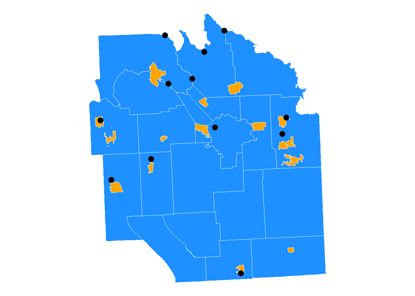
We can see that many WWTPs fall within village or town boundaries. This should help us differentiate the plants that serve different communities. We can also ask the municipalities and local WWTP operators to learn more, but for now, let us assume that we are not sure.
3.4.4 Step 4 - Filter the parcel data for public sewer only
There are two fields in the data for sewer. One is the SEWER_TYPE and the other is SEWER_DESC. SEWER_DESC includes three categories: Comm/public, None, or Private. We will filter for the Comm/public sewer parcels only.
# filter for public sewer parcels
table(onondaga_parcels$SEWER_DESC)
##
## Comm/public None Private
## 138461 11440 30452onondaga_sewer <- onondaga_parcels %>%
filter(SEWER_DESC == "Comm/public")
# plot the parcel data
# NOTE - this will take a moment, there are over 100,000 records
ggplot()+
geom_sf(data = onondaga_border, fill = NA)+
geom_sf(data = onondaga_towns, fill = "dodgerblue", color = "white")+
geom_sf(data = onondaga_villages, fill = "orange", color = "white")+
geom_sf(data = onondaga_sewer, color = NA, alpha = 0.5)+
geom_sf(data = wwtp_onondaga_sf, color = "black", size = 3)+
theme_void()+
labs(title = "Onondaga county parcels connected to public sewer")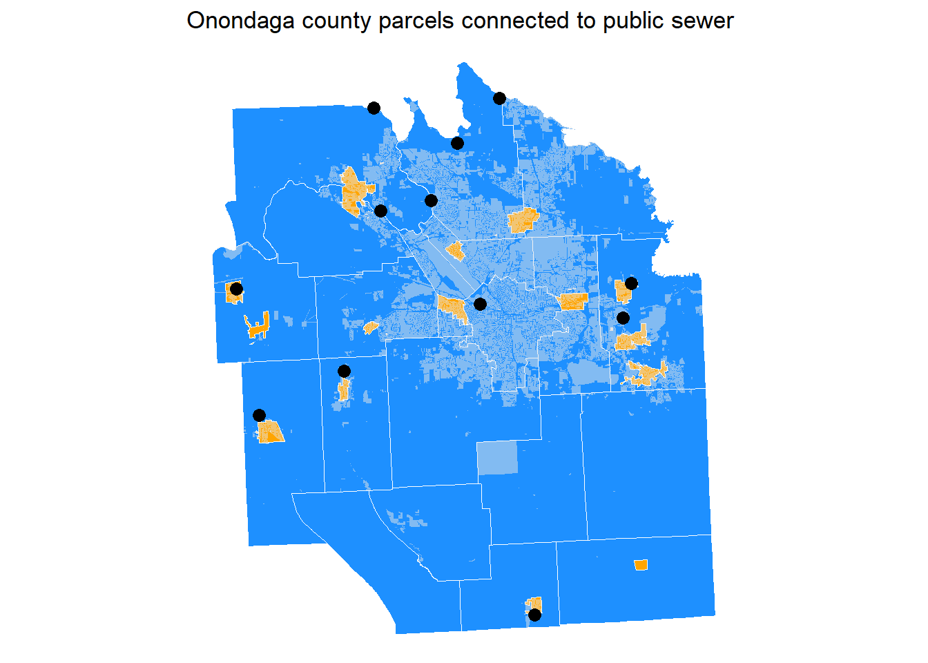
3.4.5 Step 5 - Link sewer parcels to towns and villages
# cut out the village boundaries from the towns
town_no_village <-st_difference(onondaga_towns, st_combine(onondaga_villages))

# intersect the villages/towns with the sewer parcels
sewer_town_intersection <- st_intersection(onondaga_sewer, town_no_village)
sewer_village_intersection <- st_intersection(onondaga_sewer, onondaga_villages)

# group by town / village unit and dissolve
# Note we are using a buffer to help remove extra spaces and lines between
# parcels

# first we buffer
dissolved_towns <- sewer_town_intersection %>%
  st_as_sf() %>%
  st_buffer(100)

# then dissolve
dissolved_towns <- dissolved_towns %>%
  group_by(NAME) %>% # name of the town
  summarise() %>%
  ungroup()

# remove the buffer distance
dissolved_towns <- dissolved_towns %>%
  st_buffer(-100)

# villages

# first we buffer
dissolved_villages <- sewer_village_intersection %>%
  st_as_sf() %>%
  st_buffer(100)

# then dissolve
dissolved_villages <- dissolved_villages %>%
  group_by(NAME) %>%
  summarise() %>%
  ungroup()

# remove the buffer distance
dissolved_villages <- dissolved_villages %>%
  st_buffer(-100)

# plot to see how they look
ggplot()+
  geom_sf(data = onondaga_border, fill = NA)+
  geom_sf(data = dissolved_towns, color = "white", aes(fill = `NAME`))+
    geom_sf(data = dissolved_villages, color = "white", aes(fill = `NAME`))+
  geom_sf(data = wwtp_onondaga_sf, size = 3, color = "black")+
  theme_void()+
  theme(legend.position = "none")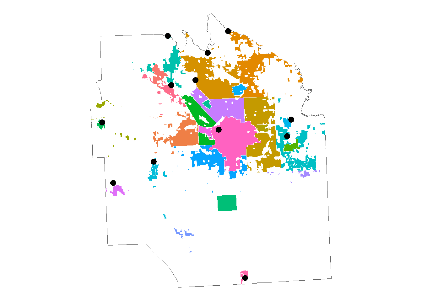
We now have two layers, parcels in each town or city that are on sewer and parcels in each village that are on sewer. The next step can be to take these data to a local county planning office and identify which town sewer systems go to each plant, then group the polygons to create the sewershed for that plant.
Alternatively, let’s do a little more work to make that next step easier. You will notice there are a lot of wayward parcels (parcels that are not near any WWTP or town and look like small “islands”). They likely flow into nearby systems a little ways off. Also, there are a lot of holes in the parcel groups. We will fill in those holes and then intersect the town and village sewer parcels with census blocks to get more robust geometries for the sewersheds. These steps will make using these data for epidemiology a little easier. If you want to keep the more skeletal boundaries for sewers, you can save that data for future reference.
3.4.5.1 Clean up sewershed boundaries
# remove holes

dissolved_towns_filled <- nngeo::st_remove_holes(dissolved_towns)
dissolved_villages_filled <- nngeo::st_remove_holes(dissolved_villages)

sewer_parcel_plot <-
  ggplot()+
  geom_sf(data = onondaga_border, fill = NA)+
  geom_sf(data = dissolved_towns_filled, color = "white", aes(fill = NAME))+
  geom_sf(data = dissolved_villages_filled, color = "white", aes(fill = NAME))+
  geom_sf(data = wwtp_onondaga_sf, size = 3, color = "black")+
  labs(title = "Town and village parcels that are on sewer")+
  theme_void()+
  theme(legend.position = "none",
        plot.title = element_text(hjust = 0.5))

sewer_parcel_plot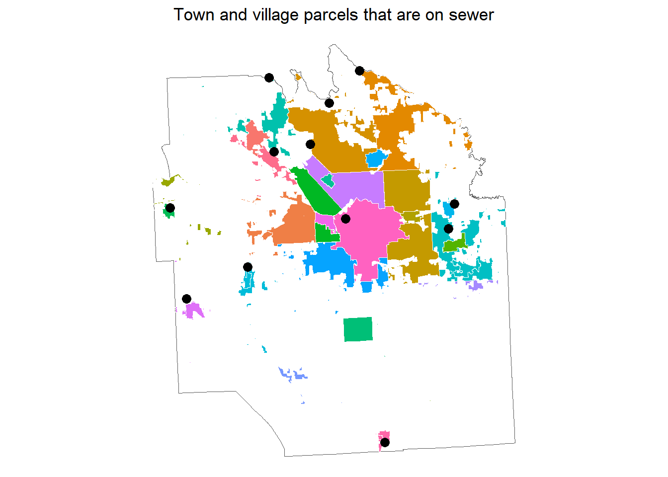
3.4.6 Step 6 - Assign polygons to WWTPs
We want to now bring our village and town parcel polygons together into one shapefile layer and link the polygons to the nearest WWTP.
# combine village and town parcels into on R data object
village_town_sewer <- bind_rows(
                                dissolved_towns_filled,
                                dissolved_villages_filled
                                )


# assign each polygon to a point based on proximity
near <- st_nearest_feature(village_town_sewer, wwtp_onondaga_sf)

# using the row numbers for the nearest feature, we can begin to create some
# sewershed boundaries
wwtp_onondaga_sf$wwtp_row_id <- seq(1:nrow(wwtp_onondaga_sf))
village_town_sewer$parcel_row_id <- seq(1:nrow(village_town_sewer))

# combine the list of near wwtps with the Onondaga sewer dataset
near_df <- as.data.frame(cbind(village_town_sewer, near))

# rename near value to be the wwtp_row_id
near_df$wwtp_row_id <- near_df$near

# to avoid extra "lines" in our dissolved polygons, we buffer the parcels first

# first we buffer
dissolved <- near_df %>%
  st_as_sf() %>%
  st_buffer(10)

# then dissolve
dissolved <- dissolved %>%
  group_by(wwtp_row_id) %>%
  summarise() %>%
  ungroup()

# remove the buffer distance
dissolved <- dissolved %>%
  st_buffer(-10)

# add the wwtp metadata
onondaga_meta <- wwtp_onondaga_sf %>%
  st_drop_geometry()

dissolved <- dissolved %>%
  left_join(onondaga_meta, by = c("wwtp_row_id"))

# plot to see how they look
ggplot()+
  geom_sf(data = onondaga_border, fill = NA)+
  geom_sf(data = dissolved, color = "darkblue", aes(fill = `Facility.Name`))+
  geom_sf(data = wwtp_onondaga_sf, size = 3, color = "black")+
  theme_void()+
  theme(legend.position = "bottom")+
  guides(fill = guide_legend(nrow = 4, byrow=TRUE))+
  scale_fill_manual(values = MetBrewer::met.brewer(name = "Nizami", n = 11),
                    labels = function(x) stringr::str_wrap(x, width = 15))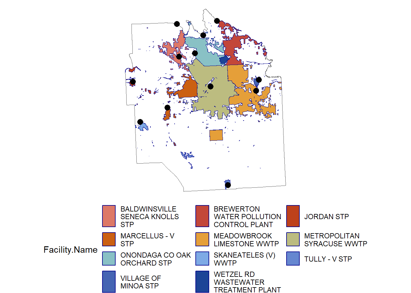
We can save these R objects as shapefiles.
st_write(dissolved_towns_filled,
         dsn = "data/onondaga town sewer parcels/onondaga town sewer parcels.shp")

st_write(dissolved_villages_filled,
         dsn = "data/onondaga village sewer parcels/onondaga village sewer parcels.shp")

st_write(dissolved,
         dsn = "data/town village sewer parcels/town village sewer parcels.shp")
3.5 Training review
We have used publicly available tax parcel data to estimate sewersheds for municipal WWTPs in Onondaga County, NY. The boundaries are not exact nor are they complete. You will need to work with local planning offices to improve the boundary estimates and finalize assigning each polygon to the WWTP that they flow into.
Some additional data you might gather to create the final boundaries include municipal tax roles, municipal sewer infrastructure maps or GIS data, or your tax parcel data might have what in NY is called a “Special Districts” table.
3.5.1 Appendix 1 - Special districts
The Special Districts table is a dataset that includes more detail on each tax parcel like what water and fire district the parcel is part of. These tables are not always publicly available and you might need permission to work with these data. If you can obtain these data, you can merge the special districts to the parcel data using the municipal tax parcel ID, and then group and filter by special district names for sewer districts. Not all special district table will have sewer data, but many will.
3.5.2 Appendix 2 - create polygons using census blocks
We can also draw sewershed boundaries using census blocks. By intersecting census blocks with sewer parcels, we can map the parts of each town and village on sewer.
An advantage to including the entire block that intersects with a sewershed parcel is that it will make merging these data with census population data easier in the future. Obtaining accurate population estimates for the number of people on sewer is an important part of wastewater-based epidemiology.
3.5.2.1 Download censusblocks for NYS
b <- tigris::blocks(state = "New York", county = "Onondaga", year = 2020)# blocks that intersect with town sewer parcels
# transform crs to match
b <- st_transform(b, st_crs(dissolved_towns_filled))
town_sewer_b <- st_intersects(b, dissolved_towns_filled)
town_sewer_b <- as.data.frame(town_sewer_b)
# blocks that intersect with village sewer parcels
village_sewer_b <- st_intersects(b, dissolved_villages_filled)
village_sewer_b <- as.data.frame(village_sewer_b)
# add row ids and then select for row ids in the intersection
b$b_row_id <- seq(1:nrow(b))
village_sewer_blocks <- b %>%
filter(b_row_id %in% village_sewer_b$row.id)
town_sewer_blocks <- b %>%
filter(b_row_id %in% town_sewer_b$row.id)
# add town / village sewer
dissolved_towns_filled$town_id <- seq(1:nrow(dissolved_towns_filled))
dissolved_villages_filled$village_id <- seq(1:nrow(dissolved_villages_filled))
village_sewer_b <- village_sewer_b %>%
rename(village_id = col.id,
b_row_id = row.id) %>%
left_join(dissolved_villages_filled, by = c("village_id")) %>%
st_drop_geometry() %>%
select(-geometry)
# add to village_sewer_blocks
village_sewer_blocks <- left_join(village_sewer_blocks, village_sewer_b,
by = c("b_row_id")
)
# group by village and dissolve
# first we buffer
village_sewer_blocks <- village_sewer_blocks %>%
st_as_sf() %>%
st_buffer(100)
# then dissolve
village_sewer_blocks <- village_sewer_blocks %>%
group_by(NAME) %>%
summarise() %>%
ungroup()
# remove the buffer distance
village_sewer_blocks <- village_sewer_blocks %>%
st_buffer(-100)
## repeat for towns
town_sewer_b <- town_sewer_b %>%
rename(town_id = col.id,
b_row_id = row.id) %>%
left_join(dissolved_towns_filled, by = c("town_id")) %>%
st_drop_geometry() %>%
select(-geometry)
# add to village_sewer_blocks
town_sewer_blocks <- left_join(town_sewer_blocks, town_sewer_b,
by = c("b_row_id")
)
# group by village and dissolve
# first we buffer
town_sewer_blocks <- town_sewer_blocks %>%
st_as_sf() %>%
st_buffer(100)
# then dissolve
town_sewer_blocks <- town_sewer_blocks %>%
group_by(NAME) %>%
summarise() %>%
ungroup()
# remove the buffer distance
town_sewer_blocks <- town_sewer_blocks %>%
st_buffer(-100)
# fill holes
town_sewer_blocks_filled <- nngeo::st_remove_holes(town_sewer_blocks)
village_sewer_blocks_filled <- nngeo::st_remove_holes(village_sewer_blocks)
block_sewer_plot <-
ggplot()+
geom_sf(data = onondaga_border, fill = NA)+
geom_sf(data = village_sewer_blocks_filled, color = "white",
aes(fill = NAME)
)+
geom_sf(data = town_sewer_blocks_filled, color = "white",
aes(fill = NAME)
)+
geom_sf(data = wwtp_onondaga_sf, size = 3, color = "black")+
labs(title = "Town and village blocks that intersect with\nparcels on sewer")+
theme_void()+
theme(legend.position = "none",
plot.title = element_text(hjust = 0.5))
# block_sewer_plotSo now we have two sets of data to bring to the local planning offices or WWTP operators to help in creating the final boundaries. Let’s take a look at them side by side.
gridExtra::grid.arrange(sewer_parcel_plot, block_sewer_plot, nrow = 1)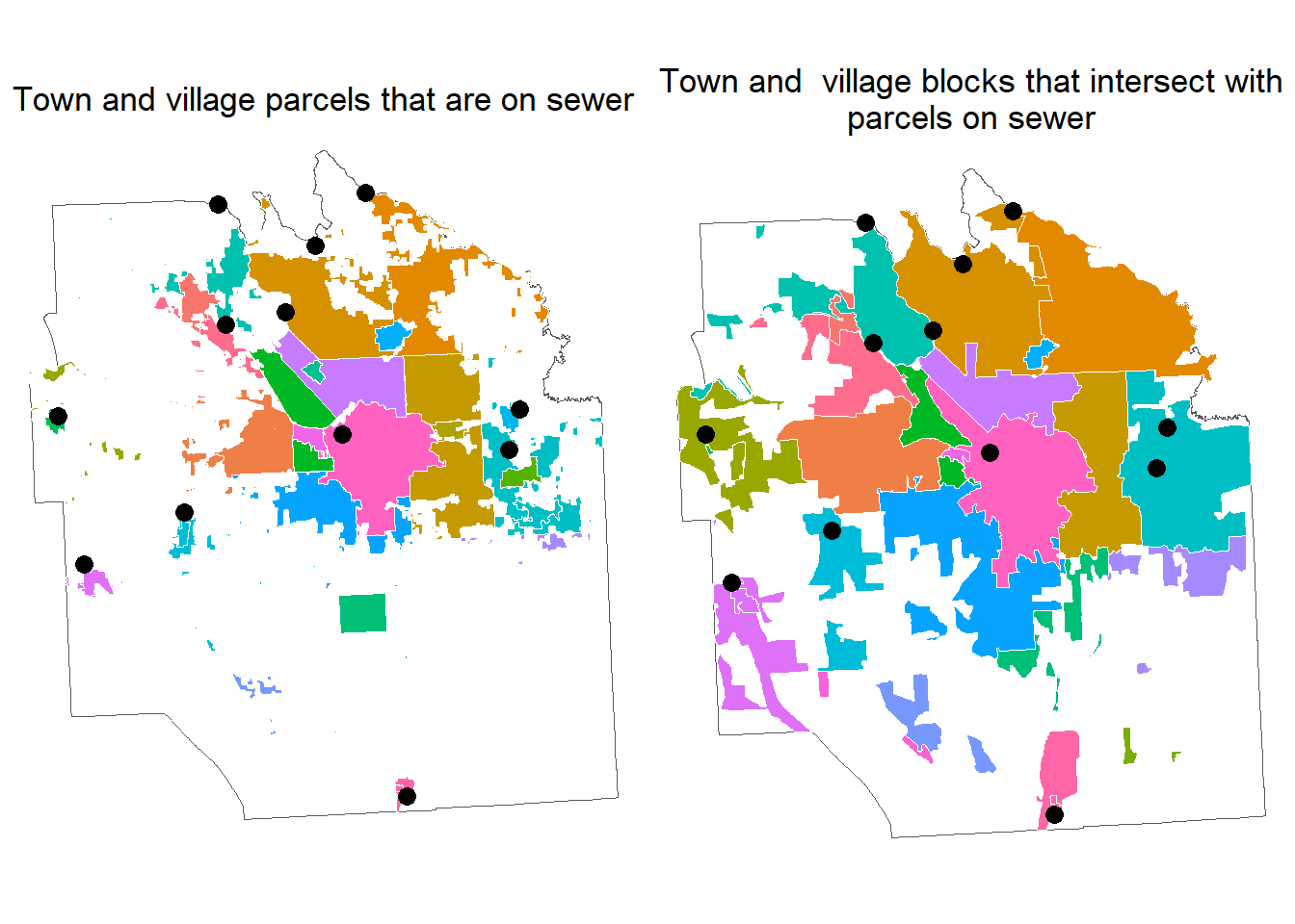
We can also link these data to the nearest WWTP like we did for parcels.
# combine into one object
village_town_blocks <- bind_rows(town_sewer_blocks, village_sewer_blocks)

# assign each polygon to a point based on proximity
near <- st_nearest_feature(village_town_blocks, wwtp_onondaga_sf)

# using the rownumbers for the nearest feature, we can begin to create some
# sewershed boundaries
wwtp_onondaga_sf$wwtp_row_id <- seq(1:nrow(wwtp_onondaga_sf))
village_town_blocks$parcel_row_id <- seq(1:nrow(village_town_blocks))

# combine the list of near wwtps with the onondaga sewer dataset
near_df <- as.data.frame(cbind(village_town_blocks, near))

# rename near value to be the wwtp_row_id
near_df$wwtp_row_id <- near_df$near

# to avoid extra "lines" in our dissolved polygons, we buffer the parcels first

# first we buffer
dissolved <- near_df %>%
  st_as_sf() %>%
  st_buffer(10)

# then dissolve
dissolved <- dissolved %>%
  group_by(wwtp_row_id) %>%
  summarise() %>%
  ungroup()

# remove the buffer distance
dissolved <- dissolved %>%
  st_buffer(-10)

# add the wwtp metadata
onondaga_meta <- wwtp_onondaga_sf %>%
  st_drop_geometry()

dissolved <- dissolved %>%
  left_join(onondaga_meta, by = c("wwtp_row_id"))

# plot to see how they look
ggplot()+
  geom_sf(data = onondaga_border, fill = NA)+
  geom_sf(data = dissolved, color = "darkblue", aes(fill = `Facility.Name`))+
  geom_sf(data = wwtp_onondaga_sf, size = 3, color = "black")+
  theme_void()+
  theme(legend.position = "none")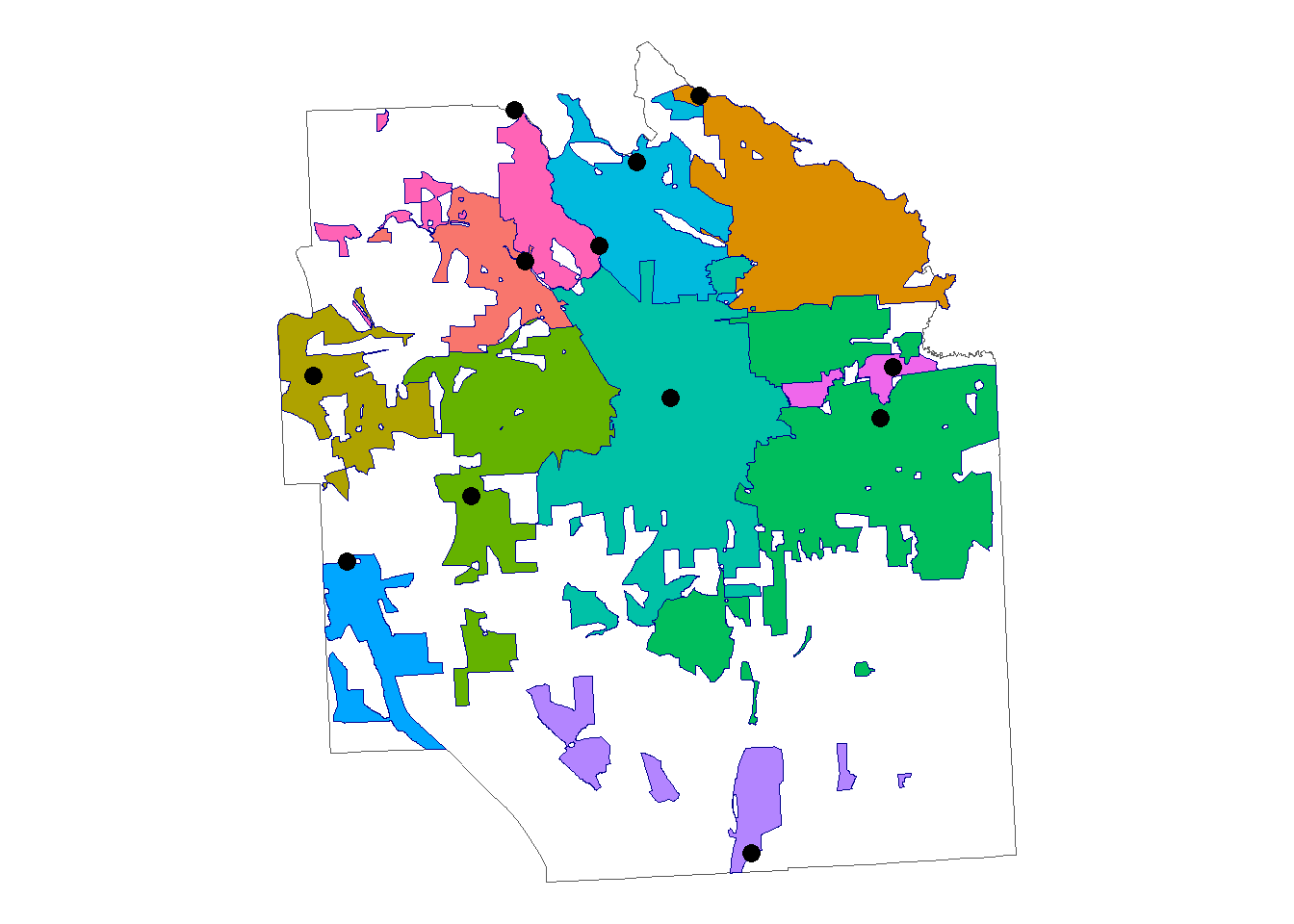
3.5.3 Appendix 3 - Polygons from point data
Some datasets may be made up of points like manhole locations or points for each parcel connected to a sewer system. You can create a polygon from point data using the following code.
# change parcels to centroids
onondaga_sewer_centroids <- st_centroid(onondaga_sewer)

# find the nearest wwtp for each sewer parcel
near <- st_nearest_feature(onondaga_sewer_centroids, wwtp_onondaga_sf)

# using the row numbers for the nearest feature, we can begin to create some
# sewershed boundaries
wwtp_onondaga_sf$wwtp_row_id <- seq(1:nrow(wwtp_onondaga_sf))
onondaga_sewer_centroids$parcel_row_id <- seq(1:nrow(onondaga_sewer_centroids))

# combine the list of near wwtps with the Onondaga sewer dataset
near_df <- as.data.frame(cbind(onondaga_sewer_centroids, near))

# rename near value to be the wwtp_row_id
near_df$wwtp_row_id <- near_df$near

# plot the points
ggplot()+
  geom_sf(data = onondaga_border, fill = NA)+
  geom_sf(data = st_as_sf(near_df), alpha = 0.5)+
  theme_void()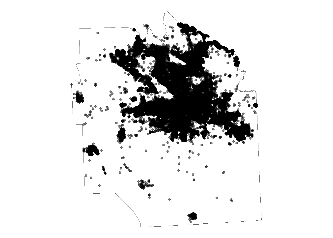
# make a buffer around each point
near_df <- near_df %>%
  st_as_sf() %>%
  st_buffer(dist = 100) # you might need to play with this buffer distance

# group by wwtp_row_id and merge into polygons
# then dissolve
dissolved <- near_df %>%
  group_by(wwtp_row_id) %>%
  summarise() %>%
  ungroup()

# plot
ggplot()+
  geom_sf(data = onondaga_border, fill = NA)+
  geom_sf(data = dissolved, aes(fill = as.factor(wwtp_row_id)))+
  geom_sf(data = wwtp_onondaga_sf, aes(size = `Average.Design.Hydraulic.Flow`))+
  theme_void()+
  theme(legend.position = "none")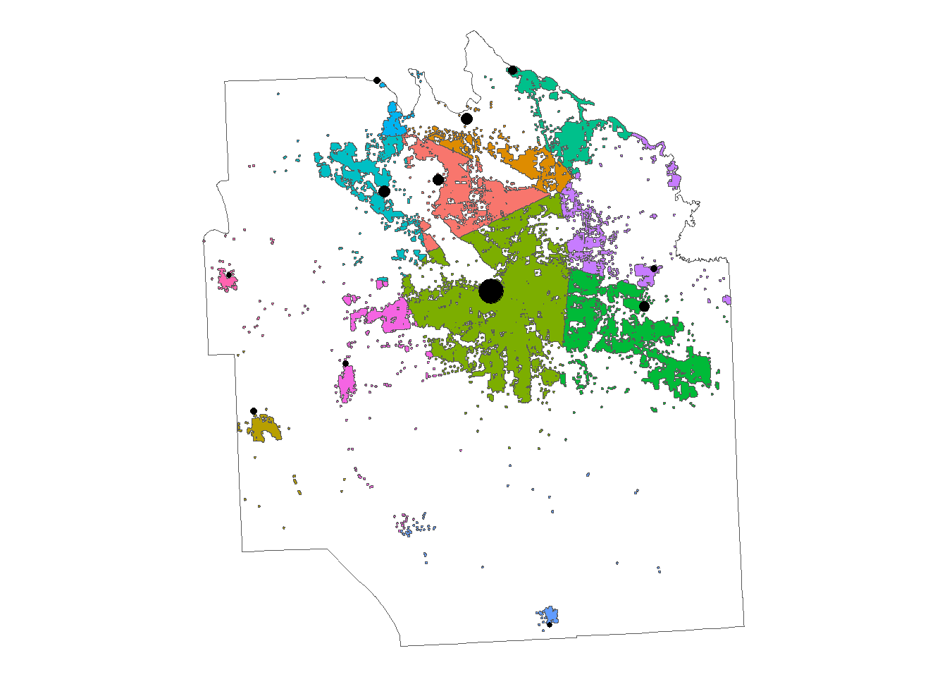
You can then fill the holes like we did before or do some additional cleaning in ArcGIS or from the special districts tables.