Chapter 4 Adding Census Data to Wastewater-Based Epidemiology
4.1 Overview
Wastewater-based epidemiology (WBE) data can be enhanced by adding other public data sources. One source is United States Census (US Census) data, which can add population demographic variables to WBE data, This vignette demonstrates how to take a spatial WBE dataset of sewershed boundaries in New York State (NYS) and add US Census data using spatial intersection methods.
4.1.1 Install and Load R packages
Install packages to your computer.
install.packages("dplyr")
install.packages("ggplot2")
install.packages("sf")
install.packages("tidycensus")
install.packages("units")
Load packages into your R session.
library(dplyr) # data wrangling
library(sf) # spatial data manipulation
library(ggplot2) # making plots and maps
library(tidycensus) # download tabular census data
library(tigris) # download spatial census data
library(tidyr) # data wrangling
library(units) # handling variables with unit assignment
4.2 Load wastewater data
Sewershed boundaries for NYS can be downloaded from ArcGIS online.
# load the boundaries
sewersheds <- st_read("data/New York State Sewersheds/New York State Sewersheds.shp")

# select the variables we want to keep
sewersheds <- sewersheds %>%
  dplyr::select(County, City, WWTP_ID, WWTP, Sewershed, SW_ID, geometry)
Map your data.
# plot to view the data
ggplot()+
  geom_sf(data = sewersheds, fill = "white", color = "black")+
  theme_void()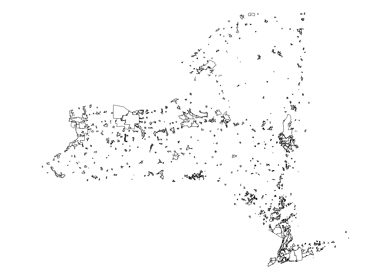
4.3 Load US Census data method - Tidy Census
US Census data can be added to your R session using the packages tidycensus and tigris. Both packages connect to the US Census API for downloading tabular data or spatial boundaries. You will need an API key to access the data. For information on obtaining a key, visit the tidycensus website.
# retrieve your API key if stored in the environment
census_api_key(Sys.getenv('CENSUS_API_KEY'))
For this example, we are going to download 2020 decennial census data and calculate the total number of individuals that self-identify as black or African American from that year. We will calculate totals and percentage of total population. We are going to use census tracts as our geography.
To download the data, we need to know the name of the variables we want and for that, we use the load_variables command.
# load the variable names into an R object. cache = TRUE can speed the data download step in the next portion
census_var_names <- load_variables(year = 2020, dataset = "pl", cache = TRUE)
# look at the first few rows of data
head(census_var_names)## # A tibble: 6 x 3
## name label concept
## <chr> <chr> <chr>
## 1 H1_001N " !!Total:" OCCUPANCY STATUS
## 2 H1_002N " !!Total:!!Occupied" OCCUPANCY STATUS
## 3 H1_003N " !!Total:!!Vacant" OCCUPANCY STATUS
## 4 P1_001N " !!Total:" RACE
## 5 P1_002N " !!Total:!!Population of one race:" RACE
## 6 P1_003N " !!Total:!!Population of one race:!!White alone" RACEThis function can load the variable names for many datasets from the US Census and provides the name, the variable description, and the concept group that the variable is part of. Looking at the options, we can see that we want a variable from the RACE concept, specifically, P1_004N, which is “!!Total:!!Population of one race:!!Black or African American alone”. For this exercise, we will not be included those that identify as multiple racial or ethnic groups, but you can adapt the methods presented to make those calculations.
To get the total for each census tract that identify as black or African American, we need this variable. However, to calculate the percent of the population, we also need the total population, which is the variable ” !!Total:” or P1_001N. We will use the get_dencennial function to download the data into our R session.
# download the decennial data for the tract geography for NYS
census_data <- get_decennial(
  year = 2020,
  geography = "tract",
  state = "New York",
  variables = c(
    c(population_total = "P1_001N"),
    black_alone = "P1_004N"
  )
)
# view the first few rows of data
head(census_data)## # A tibble: 6 x 4
## GEOID NAME variable value
## <chr> <chr> <chr> <dbl>
## 1 36001000100 Census Tract 1, Albany County, New York population_total 2073
## 2 36001000201 Census Tract 2.01, Albany County, New York population_total 3125
## 3 36001000202 Census Tract 2.02, Albany County, New York population_total 2598
## 4 36001000301 Census Tract 3.01, Albany County, New York population_total 3190
## 5 36001000302 Census Tract 3.02, Albany County, New York population_total 3496
## 6 36001000401 Census Tract 4.01, Albany County, New York population_total 2216The resulting dataset is now in our R session with 10,822 rows. We will need to pivot the dataframe to a wider format because it placed the variables in a long format.
# pivot the data from long to wide format
census_data <- pivot_wider(census_data,
                           names_from = variable)

# summary of the dataset variables
summary(census_data)
## GEOID NAME population_total black_alone
## Length:5411 Length:5411 Min. : 0 Min. : 0.0
## Class :character Class :character 1st Qu.: 2490 1st Qu.: 47.5
## Mode :character Mode :character Median : 3578 Median : 164.0
## Mean : 3733 Mean : 551.9
## 3rd Qu.: 4762 3rd Qu.: 667.0
## Max. :17222 Max. :7935.0Now we have census counts for individuals that self-identify as black or African American and we want to add these data to our wastewater sewershed boundaries. To do this, we need to add the census geometry (the spatial component) to the R session.
# download tracts for NY for 2020 and drop the name column
tracts <- tracts(state = "New York", year = 2020) %>% select(-NAME)

# join the tract geometries to the census data
census_data_sf <- left_join(tracts, census_data, by = c("GEOID"))
# check the data structure
str(census_data_sf)## Classes 'sf' and 'data.frame': 5411 obs. of 15 variables:
## $ STATEFP : chr "36" "36" "36" "36" ...
## $ COUNTYFP : chr "047" "047" "047" "047" ...
## $ TRACTCE : chr "000700" "000900" "001100" "001300" ...
## $ GEOID : chr "36047000700" "36047000900" "36047001100" "36047001300" ...
## $ NAMELSAD : chr "Census Tract 7" "Census Tract 9" "Census Tract 11" "Census Tract 13" ...
## $ MTFCC : chr "G5020" "G5020" "G5020" "G5020" ...
## $ FUNCSTAT : chr "S" "S" "S" "S" ...
## $ ALAND : num 176774 163469 168507 293167 154138 ...
## $ AWATER : num 0 0 0 0 0 ...
## $ INTPTLAT : chr "+40.6923505" "+40.6917206" "+40.6932903" "+40.6976150" ...
## $ INTPTLON : chr "-073.9973434" "-073.9916018" "-073.9877087" "-073.9883586" ...
## $ NAME : chr "Census Tract 7, Kings County, New York" "Census Tract 9, Kings County, New York" "Census Tract 11, Kings County, New York" "Census Tract 13, Kings County, New York" ...
## $ population_total: num 4415 5167 1578 2465 1694 ...
## $ black_alone : num 151 197 178 234 172 ...
## $ geometry :sfc_MULTIPOLYGON of length 5411; first list element: List of 1
## ..$ :List of 1
## .. ..$ : num [1:35, 1:2] -74 -74 -74 -74 -74 ...
## ..- attr(*, "class")= chr [1:3] "XY" "MULTIPOLYGON" "sfg"
## - attr(*, "sf_column")= chr "geometry"
## - attr(*, "agr")= Factor w/ 3 levels "constant","aggregate",..: NA NA NA NA NA NA NA NA NA NA ...
## ..- attr(*, "names")= chr [1:14] "STATEFP" "COUNTYFP" "TRACTCE" "GEOID" ...4.4 Adding the Census data to the wastewater data
4.4.1 Spatial transformations
To add our population data to the sewershed data, we have a few steps to complete. First, both of our datasets need to be the same spatial projection so that they spatially overlap and can be mapped on top of each other.
# transform the census data CRS to match the sewersheds
census_data_sf <- st_transform(census_data_sf, st_crs(sewersheds))

# plot the data, the layers should overlap
ggplot()+
  geom_sf(data = census_data_sf, fill = "white", color = "black")+
  geom_sf(data = sewersheds, fill = "blue", color = "black")+
theme_void()![]()
4.4.2 Spatial intersection
Now we want to spatially intersect the data. This will assign census count data to the sewersheds that overlap. Sewershed boundaries do not follow census tract boundaries closely, so we have two options for assigning the data. First, we can apportion census data to the sewersheds using the proportion of each census tract area that is within the sewershed area. Alternatively, we can assign the total population for all intersecting tracts to the sewershed.
The first method, called areal apportionment, is generally thought to provide more accurate methods for counts of the data, but assumes that people are evenly distributed within the census tract. The second method could be useful if it is not known how evenly the population is distributed and you want to avoid excluding anyone. We will practice both methods.
4.4.2.1 Areal apportionment
# calculate the area of each census tract. Note this field becomes a unit
# variable, we will have to drop those later
census_data_sf$tract_area <- st_area(census_data_sf)

# turn of spherical geometry to handle overlapping edges and invalid vertices
# warnings
sf::sf_use_s2(FALSE)

# intersect both datasets, creating a new dataset that has slivers of each tract
# that intersects a sewershed
intersection <- st_intersection(sewersheds, census_data_sf)

summary(intersection)
## County City WWTP_ID WWTP
## Length:7963 Length:7963 Length:7963 Length:7963
## Class :character Class :character Class :character Class :character
## Mode :character Mode :character Mode :character Mode :character
##
##
##
## Sewershed SW_ID STATEFP COUNTYFP
## Length:7963 Length:7963 Length:7963 Length:7963
## Class :character Class :character Class :character Class :character
## Mode :character Mode :character Mode :character Mode :character
##
##
##
## TRACTCE GEOID NAMELSAD MTFCC
## Length:7963 Length:7963 Length:7963 Length:7963
## Class :character Class :character Class :character Class :character
## Mode :character Mode :character Mode :character Mode :character
##
##
##
## FUNCSTAT ALAND AWATER INTPTLAT
## Length:7963 Min. :0.000e+00 Min. :0.000e+00 Length:7963
## Class :character 1st Qu.:2.136e+05 1st Qu.:0.000e+00 Class :character
## Mode :character Median :1.176e+06 Median :0.000e+00 Mode :character
## Mean :1.933e+07 Mean :2.107e+06
## 3rd Qu.:6.154e+06 3rd Qu.:1.536e+05
## Max. :1.828e+09 Max. :1.997e+09
## INTPTLON NAME population_total black_alone
## Length:7963 Length:7963 Min. : 0 Min. : 0.0
## Class :character Class :character 1st Qu.: 2593 1st Qu.: 61.0
## Mode :character Mode :character Median : 3672 Median : 211.0
## Mean : 3803 Mean : 587.3
## 3rd Qu.: 4824 3rd Qu.: 734.5
## Max. :17222 Max. :7935.0
## tract_area geometry
## Min. :2.169e+04 GEOMETRYCOLLECTION: 28
## 1st Qu.:2.261e+05 MULTIPOLYGON :1583
## Median :1.277e+06 POLYGON :6352
## Mean :2.140e+07 epsg:4269 : 0
## 3rd Qu.:6.565e+06 +proj=long... : 0
## Max. :1.993e+09Our spatial data are now combined into one spatial data object.
# calculate a new area for each sliver
intersection$sliver_area <- st_area(intersection)

# calculate the proportion of area that each sliver occupies in the sewershed
intersection$prop_area <- intersection$sliver_area / intersection$tract_area
summary(intersection$prop_area)
## Min. 1st Qu. Median Mean 3rd Qu. Max.
## 0.00000 0.06113 0.88439 0.60984 1.00122 1.00216# You will notice some areas are slightly over 1 representing a rounding error. Let's make those all 1 to avoid assignment issues
# drop units
intersection$prop_area <- drop_units(intersection$prop_area)
intersection$prop_area <- ifelse(intersection$prop_area > 1,
1,
intersection$prop_area
)
summary(intersection$prop_area)## Min. 1st Qu. Median Mean 3rd Qu. Max.
## 0.00000 0.06113 0.88439 0.60930 1.00000 1.00000# multiply the proportional area by the totals for black or African American and total population to get proportional values
intersection$prop_black <- intersection$prop_area * intersection$black_alone
intersection$prop_population <-
intersection$prop_area * intersection$population_total
# how we will group the data by sewershed and sum the total population and total black population in each sewershed
intersection_final <- intersection %>%
group_by(County, City, WWTP_ID, WWTP, Sewershed, SW_ID) %>%
summarize(sum_black_alone = sum(prop_black, na.rm = TRUE),
sum_total_population = sum(prop_population)
) %>%
ungroup()
# our resulting dataset has 674 rows, one for each sewershed, and proportional estimates for population totals and the total number of individuals that self identify as black or African American
summary(intersection_final)## County City WWTP_ID WWTP
## Length:674 Length:674 Length:674 Length:674
## Class :character Class :character Class :character Class :character
## Mode :character Mode :character Mode :character Mode :character
##
##
##
## Sewershed SW_ID sum_black_alone sum_total_population
## Length:674 Length:674 Min. : 0.00 Min. : 0.2
## Class :character Class :character 1st Qu.: 0.74 1st Qu.: 66.6
## Mode :character Mode :character Median : 12.91 Median : 595.6
## Mean : 4932.45 Mean : 27214.5
## 3rd Qu.: 381.10 3rd Qu.: 7356.8
## Max. :307461.96 Max. :1154606.8
## geometry
## GEOMETRYCOLLECTION: 2
## MULTIPOLYGON :160
## POLYGON :512
## epsg:4269 : 0
## +proj=long... : 0
## We have estimated totals, which can be useful, but often, percentage of the population is more informative for analyses. We can get an estimated proportion of the population by dividing the total black alone variable by the total population value.Also, you will notice that the values are no longer integers, meaning that there are estimates for total number of people that include decimals. These can be rounded to the nearest whole number to return the data back to integers.
# calculate the proportion
intersection_final$prop_black <-
  intersection_final$sum_black_alone / intersection_final$sum_total_population

# plot the percentages
ggplot()+
  geom_sf(data = intersection_final, aes(fill = prop_black), color = "black")+
  theme_void()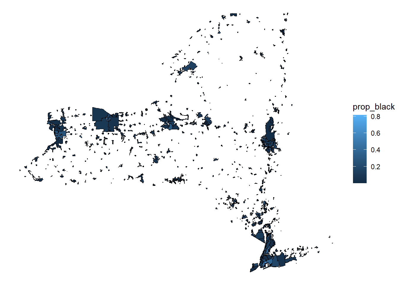
4.4.2.2 Intersection assignment
The other method for assigning data is to assign the total population for all census tracts that intersect with a sewershed.
# st_intersects returns a list of the polygon rows that intersect from each
# object
intersect_list <- st_intersects(sewersheds, census_data_sf)
# make it a dataframe
intersect_df <- as.data.frame(intersect_list)
# view the top view rows
head(intersect_df)## row.id col.id
## 1 1 1142
## 2 1 1145
## 3 1 1146
## 4 1 2664
## 5 1 3692
## 6 1 5333Column 1 are the row ids for the sewersheds and column 2 are the row ids for the tracts that intersect them. We will add the row ids to each data object, then use those to merge the census counts to the spatial data and sum to totals.
# add row ids
sewersheds$sewer_row_id <- as.integer(rownames(sewersheds))
census_data_sf$census_row_id <- as.integer(rownames(census_data_sf))


# rename intersect column and merge to spatial sewersheds
colnames(intersect_df) <- c("sewer_row_id", "census_row_id")
intersect_combined <- full_join(sewersheds, intersect_df,
                                by = c("sewer_row_id")
                                )

# change the census data from a spatial object to a dataframe
census_data_df <- st_drop_geometry(census_data_sf)

# merge census data -> note that we have to remove the spatial data from the
# census data
intersect_combined <- left_join(intersect_combined, census_data_df,
                                by = c("census_row_id")
                                )

# sum the total number of people that are in census tracts intersecting each
# sewershed
intersect_final <- intersect_combined%>%
  group_by(County, City, WWTP_ID, WWTP, Sewershed, SW_ID) %>%
  summarize(sum_black_alone = sum(black_alone, na.rm = TRUE),
            sum_total_population = sum(population_total, na.rm = TRUE)
            ) %>%
  ungroup()

# calculate the proportions
intersect_final$prop_black <-
  intersect_final$sum_black_alone / intersect_final$sum_total_population

# make a map
ggplot()+
  geom_sf(data = intersect_final, aes(fill = prop_black), color = "black")+
  theme_void()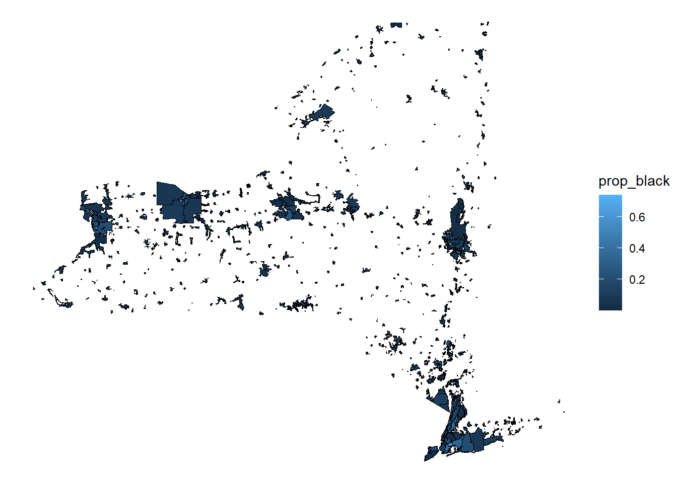
4.5 Training review
This tutorial demonstrated a process for adding US Census data to WBE spatial data (sewersheds). We calculated the percentage of each sewershed population that identified as black or African American in the 2020 decennial census. These methods can be used to estimate other data available from the US Census. For more information visit the US Census website or tidycensus.